What is Vibration?
DLI Engineering
So, let’s get into it. What is vibration?
In its simplest form, vibration can be considered to be the oscillation or repetitive motion of an object around an equilibrium position. The equilibrium position is the position the object will attain when the force acting on it is zero. This type of vibration is called “whole body motion”, meaning that all parts of the body are moving together in the same direction at any point in time.
The vibratory motion of a whole body can be completely described as a combination of individual motions of six different types. These are translation in the three orthogonal directions x, y, and z, and rotation around the x, y, and z-axes. Any complex motion the body may have can be broken down into a combination of these six motions. Such a body is therefore said to possess six degrees of freedom. For instance, a ship can move in the fore and aft direction (surge), up and down direction (heave), and port and starboard direction (sway), and it can rotate lengthwise (roll), rotate around the vertical axis (yaw), and rotate about the port-starboard axis (pitch).
Suppose an object were restrained from motion in any direction except one. For instance, a clock pendulum is restricted from motion except in one plane. It is therefore called a single degree of freedom system. Another example of a single degree of freedom system is an elevator moving up and down in an elevator shaft.
The vibration of an object is always caused by an excitation force. This force may be externally applied to the object, or it may originate inside the object. It will be seen later that the rate (frequency) and magnitude of the vibration of a given object is completely determined by the excitation force, direction, and frequency. This is the reason that vibration analysis can determine the excitation forces at work in a machine. These forces are dependent upon the machine condition, and knowledge of their characteristics and interactions allows one to diagnose a machine problem.
Energy and Power Considerations
Energy is required to produce vibration and in the case of machine vibration, this energy comes from the source of power to the machine. This energy source can be the AC power line, an internal combustion engine, or steam driving a turbine, etc. Energy is defined as force multiplied by the distance over which the force acts, and the SI unit of energy is the Joule. One Joule of energy is equivalent to a force of one Newton acting over a distance of one meter. The physical concept of work is similar to that of energy, and the units used to measure work are the same as those for measuring energy.
The actual amount of energy present in the machine vibration itself is usually not very great compared to the energy required to operate the machine for its intended task.
Power is defined as the rate of doing work, or the rate of energy transfer, and according to the SI, it is measured in Joules per second, or Watts. One horsepower is equivalent to 746 watts. Power is proportional to the square of the vibration amplitude, just as electrical power is proportional to the voltage squared or the current squared.
According to the law of conservation of energy, energy cannot be created or destroyed, but it can be transformed into different forms. The vibratory energy in a mechanical system is ultimately dissipated in the form of heat.
Linear and Non-Linear Systems
To assist in understanding the transmission of vibration through a machine, it is instructive to investigate the concept of linearity and what is meant by linear and non-linear systems. Thus far, we have discussed linear and logarithmic amplitude and frequency scales, but the term “linear” also refers to the characteristics of a system which can have input and output signals. A “system” is any device or structure that can accept an input or stimulus in some form and produce a corresponding output or response. Examples of systems are tape recorders and amplifiers, which operate on electrical signals, and mechanical structures, whose inputs are vibration forces, and whose outputs are vibration displacements, velocities, or accelerations.
Frequency Analysis
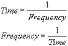
To get around the limitations in the analysis of the wave form itself, the common practice is to perform frequency analysis, also called spectrum analysis, on the vibration signal. The time domain graph is called the waveform, and the frequency domain graph is called the spectrum. Spectrum analysis is equivalent to transforming the information in the signal from the time domain into the frequency domain. The following relationships hold between time and frequency:
A train schedule shows the equivalence of information in the time and frequency domains:
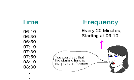
The frequency representation in this case is much shorter than the time representation. This is a “data reduction”.
Note that the information is the same in both domains, but that it is much more compact in the frequency domain. A very long schedule in time has been compressed to two lines in the frequency domain. It is a general rule of the transformation characteristic that events that take place over a long time interval are compressed to specific locations in the frequency domain.
Logarithmic Frequency Scaling
So far, the only type of frequency analysis discussed has been on a linear frequency scale, i.e., the frequency axis is set out in a linear fashion. This is suitable for frequency analysis with a frequency resolution that is constant throughout the frequency range, commonly called “narrow band” analysis. The FFT analyzer performs this type of analysis.
There are several situations where frequency analysis is desired, but narrow band analysis does not present the data in its most useful form. An example of this is acoustic noise analysis where the annoyance value of the noise to a human observer is being studied. The human hearing mechanism is responsive to frequency ratios rather than actual frequencies. The frequency of a sound determines its pitch as perceived by a listener, and a frequency ratio of two is a perceived pitch change of one octave, no matter what the actual frequencies are. For instance if a sound of 100 Hz frequency is raised to 200 Hz, its pitch will rise one octave, and a sound of 1000 Hz, when raised to 2000 Hz, will also rise one octave in pitch. This fact is so precisely true over a wide frequency range that it is convenient to define the octave as a frequency ratio of two, even though the octave itself is really a subjective measure of a sound pitch change.
This phenomenon can be summarized by saying that the pitch perception of the ear is proportional to the logarithm of frequency rather than to frequency itself. Therefore, it makes sense to express the frequency axis of acoustic spectra on a log frequency axis, and this is almost universally done. For instance, the frequency response curves that sound equipment manufacturers publish are always plotted in log frequency. Likewise, when frequency analysis of sound is performed, it is very common to use log frequency plots.
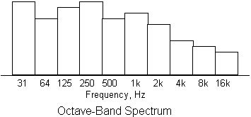
The vertical axis of an octave band spectrum is usually scaled in dB.
The octave is such an important frequency interval to the ear that so-called octave band analysis has been defined as a standard for acoustic analysis. The figure below shows a typical octave band spectrum where the ISO standard center frequencies of the octave bands are used. Each octave band has a bandwidth equal to about 70% of it center frequency. This type of spectrum is called constant percentage band because each frequency band has a width that is a constant percentage of its center frequency. In other words, the analysis bands become wider in proportion to their center frequencies.
It can be argued that the frequency resolution in octave band analysis is too poor to be of much use, especially in analyzing machine vibration signatures, but it is possible to define constant percentage band analysis with frequency bands of narrower width. A common example of this is the one-third-octave spectrum, whose filter bandwidths are about 27 % of their center frequencies. Three one-third octave bands span one octave, so the resolution of such a spectrum is three times better than the octave band spectrum. One-third octave spectra are frequently used in acoustical measurements.
A major advantage of constant percentage band analysis is that a very wide frequency range can be displayed on a single graph and the frequency resolution at the lower frequencies can still be fairly narrow. Of course, the frequency resolution at the highest frequencies suffers, but this is not a problem for some applications such as fault detection in machines.
In the chapter on machine fault diagnosis, it will be seen the narrow band spectra are very useful in resolving higher-frequency harmonics and sidebands, but for the detection of a machine fault, no such high resolution is required. The vibration velocity spectra of most machines will be found to slope downwards at the highest frequencies, and a constant percentage band (CPB) spectrum of the same data will usually be more uniform in level over a broad frequency range. This means that a CPB spectrum takes better advantage of the dynamic range of the instrumentation. One-third octave spectra are sufficiently narrow at low frequencies to show the first few harmonics of run speed, and can be used effectively for the detection of faults if trended over time.
The use of constant CPB spectra for machine monitoring is not very well recognized in industry with a few notable exceptions such as the US Navy submarine fleet.
Logarithmic Amplitude Scaling
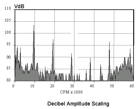
The spectrum above plots the logarithm of the vibration level rather than the level itself.
Since this spectrum is on a log amplitude scale, multiplication by any constant value simply translates the spectrum up on the screen without changing its shape or the relationship between the components.
Multiplication of the signal level translates into addition on a log scale. This means that if the amount of amplification of a vibration signal is changed, the shape of the spectrum is not affected. This fact greatly simplifies visual interpretation of log spectra taken at different amplification factors — the curves are simply translated up or down on the graph. With a linear scaling, the shape of the spectrum changes drastically with different degrees of amplification.
The next spectrum is presented in decibels, a special type of log scaling that is very important in vibration analysis
Linear and Logarithmic Amplitude Scales
It may seem to be best to look at vibration spectra with a linear amplitude scale because that is a true representation of the actual measured vibration amplitude. Linear amplitude scaling makes the largest components in a spectrum very easy to see and to evaluate, but very small components may be overlooked completely, or are at best difficult to assign a magnitude to. The eye is able to see small components about 1/50th as large as the largest ones in the same spectrum, but anything smaller than this is essentially lost. In other words, the dynamic range of the eye is about 50 to 1
Linear scaling may be adequate in cases where the components are all about the same size, but in the case of machine vibration, beginning faults in such parts as bearings produce very small signal amplitudes. If we are to do a good job of trending the levels of these spectral components, it is best to plot the logarithm of the amplitude rather than the amplitude itself. In this way, we can easily display and visually interpret a dynamic range of at least 5000 to 1, or more than 100 times better than the linear scaling allows.
To illustrate different types of amplitude presentations, the same vibration signature will be shown in linear and two different types of logarithmic amplitude scales.
It might be said that the dynamic range of the eye, when looking at linear spectra, is about 34 dB.
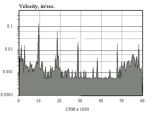
Linear Amplitude Scaling
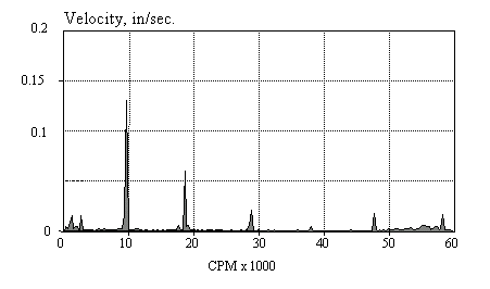
Note that this linear spectrum shows the larger peaks very well, but lower level information is missing. In the case of machine vibration analysis, we are often interested in the smaller components of the spectrum, i.e., in the case of rolling element bearing diagnosis. This subject will be covered in detail in the chapter on Machine Vibration Monitoring.
The Decibel
The decibel (dB) is defined by the following expression:
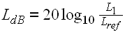
where: LdB = The signal level in dB L1 = Vibration level in Acceleration, Velocity, or Displacement
Lref = Reference level, equivalent to 0 dB
The Bell Telephone Labs introduced the concept of the decibel before 1930. It was first used to measure relative power loss and signal to noise ratio in telephone lines. It was soon pressed into service as a measure of acoustic sound pressure level.
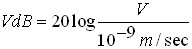
The vibration velocity level in dB is abbreviated VdB, and is defined as:
![]() or
or
The Systeme Internationale, or SI, is the modern replacement for the metric system.
The reference, or “0 dB” level of 10-9 meter per sec is sufficiently small that all our measurements on machines will result in positive dB numbers. this standardized reference level uses the SI, or “metric,” system units, but it is not recognized as a standard in the US and other English-speaking countries. (The US. Navy and many American industries use a zero dB reference of 10-8 m/sec, making their readings higher than SI readings by 20 dB.)
The VdB is a logarithmic scaling of vibration magnitude, and it allows relative measurements to be easily made. Any increase in level of 6 dB represents a doubling of amplitude, regardless of the initial level. In like manner, any change of 20 dB represents a change in level by a factor of ten. Thus any constant ratio of levels is seen as a certain distance on the scale, regardless of the absolute levels of the measurements. This makes it very easy to evaluate trended vibration spectral data; 6 dB increases always indicate doubling of the magnitudes.
dB Values vs. Amplitude Level Ratios
The following table relates dB values to amplitude ratios:
| dB Change | Linear Level Ratio | dB Change | Linear Level Ratio |
| 0 | 1 | 30 | 31 |
| 3 | 1.4 | 36 | 60 |
| 6 | 2 | 40 | 100 |
| 10 | 3.1 | 50 | 310 |
| 12 | 4 | 60 | 1000 |
| 18 | 8 | 70 | 3100 |
| 20 | 10 | 80 | 10,000 |
| 24 | 16 | 100 | 100,000 |
It is strongly recommended that VdB be used as the vibration amplitude scaling because so much more information is available to the viewer compared to linear amplitude units. Also, compared to a conventional log scale, the dB scale is much easier to read.
Unit Conversions
Acceleration and Displacement can also be expressed on dB scales. The AdB scale is the most used one, and its zero reference is set 1 micro G, commonly abbreviated G.
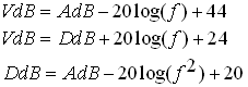
It turns out that AdB = VdB at 159.2 Hz. VdB levels, AdB levels, and DdB levels are related by the following formulas:
Any vibration parameter — displacement, velocity, or acceleration can be displayed on a dB scale. The reference quantities for 0 dB on these scales were chosen such that the dB levels of all three quantities are the same at a frequency of 159.2 Hz, which is equal to 1000 radians per second.
Acceleration and Velocity in linear units are calculated from dB levels as follows:
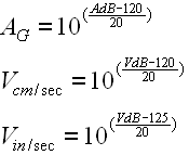
It is convenient to remember the following rule of thumb: At 100 Hz, 1G = 120 AdB = 124 VdB = 2.8 mils p-p.
Note that the time domain wave form is always represented in linear amplitude units – it is not possible to use a log scale in the wave form plot because some of the values are negative, and the logarithm of a negative number is not defined.
VdB Levels vs. Vibration Levels in ips
Peak level is the de facto standard unit for vibration velocity measurements, even though RMS level would make more sense in most cases.
Following is a convenient conversion table for relating VdB levels to inches per second peak:
| VdB | ips peak | VdB | ips peak | VdB | ips peak |
| 60 | .0006 | 90 | .018 | 120 | .56 |
| 62 | .0007 | 92 | .022 | 122 | .70 |
| 64 | .0009 | 94 | .028 | 124 | .88 |
| 66 | .0011 | 96 | .035 | 126 | 1.1 |
| 68 | .0014 | 98 | .044 | 128 | 1.4 |
| 70 | .0018 | 100 | .056 | 130 | 1.8 |
| 72 | .0022 | 102 | .070 | 132 | 2.2 |
| 74 | .0028 | 104 | .088 | 134 | 2.8 |
| 76 | .0035 | 106 | .11 | 136 | 3.5 |
| 78 | .0044 | 108 | .14 | 138 | 4.4 |
| 80 | .0056 | 110 | .18 | 140 | 5.6 |
| 82 | .0070 | 112 | .22 | 142 | 7.0 |
| 84 | .0088 | 114 | .28 | 144 | 8.8 |
| 86 | .011 | 116 | .35 | 146 | 11.1 |
| 88 | .014 | 118 | .44 | 148 | 14.0 |
Related Articles

Growing Reliability Down on the Wind Farm
Gearbox Diagnostics Fault Detection

Data Analysis Tip 3 – Compare Identical Machines

Gaps in Your Electric Motor Reliability Program

Vibration & Ultrasound Technologies: A Possible Integrated Inspection Tool?

Vibration Standards and Damage Factors for Machinery